The fastest way to run FTW field boundary detection is in your browser — no install, no code. Draw a region anywhere on the map, pick a model, and the app runs inference on Sentinel-2 imagery for that area. Results download as GeoParquet or GeoJSON for use in any GIS. The Explorer App runs the same FTW baseline models as the command-line workflow below.

This tutorial walks through downloading a pair of Sentinel-2 scenes, running an FTW Baseline model on them, and producing fiboa-compliant GeoParquet output. It works anywhere in the world; we'll use a small area in Austria as the example. The video below shows the process end to end:

Note: the video above shows the older v1/v2 workflow where model checkpoints were downloaded manually. The current CLI (shown below) uses a central model registry — the commands are structurally the same, but you reference models by name instead of by a local .ckpt file.

Choosing a Model

FTW Baselines ships with a central model registry, so you don't need to download checkpoints manually — the CLI fetches them on demand by name. Browse the available models with:

ftw model list
ftw model show FTW_PRUE_EFNET_B5

The current default is FTW_PRUE_EFNET_B5, part of the FTW v3 (PRUE) release — a three-class (field, boundary, background) U-Net with an EfficientNet-B5 encoder that balances speed and accuracy. B3 is faster, B7 is slower but more accurate. Each PRUE variant comes in two flavors:

• Standard (e.g. FTW_PRUE_EFNET_B5) — trained on the full FTW corpus including CC-BY-NC-SA and other open sources. Generally best accuracy.
• CC-BY (e.g. FTW_PRUE_EFNET_B5_CCBY) — trained only on CC-BY or CC0 data if you need clean IP provenance.

Per-dataset licensing is documented at the bottom of the FTW data homepage on Source Cooperative. Legacy v1 / v2 models and the alternative Delineate Anything instance-segmentation model are also available via the registry; see ftw model list for the full catalog. You can also train your own models on a custom dataset subset.

Fast Path: End-to-End in One Command

For most cases, ftw inference all handles the whole pipeline in a single call — it selects Sentinel-2 scenes from the USDA crop calendar for the target year, downloads them, runs inference, and polygonizes the output:

ftw inference all \
--bbox 13.0,48.0,13.2,48.2 \
--year 2024 \
--out austria-output \
--model FTW_PRUE_EFNET_B5 \
--gpu 0 \
--overwrite

This writes three files into the output directory: inference_data.tif (stacked Sentinel-2 imagery), inference_output.tif (raw segmentation raster), and polygons.parquet (fiboa-compliant field boundaries). Set --gpu -1 to run on CPU, or pass --mps_mode on Apple Silicon. If this is all you need, skip ahead to the summary.

Step-by-Step: Manual Scene Selection

If you want more control — picking specific Sentinel-2 STAC IDs rather than letting the crop calendar choose — run the pipeline in three stages.

1. Download the Data

First, fetch a pair of Sentinel-2 scenes for your planting and harvest windows. The command below writes an 8-band stacked GeoTIFF to austria.tif:

ftw inference download \
--win_a S2B_MSIL2A_20210617T100559_R022_T33UUP_20210624T063729 \
--win_b S2B_MSIL2A_20210925T101019_R022_T33UUP_20210926T121923 \
-f -o austria.tif --bbox 13.0,48.0,13.3,48.3

Bands 1–4 are RGB + NIR for Window A; bands 5–8 are the same for Window B. Use the Planetary Computer Explorer to find candidate scenes. To choose the two windows, consult the USDA crop calendar for the planting and harvest periods of your target region. For example, the China calendar shows most crops planted Feb–May and harvested Aug–Nov. Set the cloud-cover filter to 10% or less and pick a clear observation covering the AOI. Pass --bbox to limit the download to a subset of each scene — without it, the tool fetches the full tiles, which takes much longer.

2. Run Inference

Pass the stacked image to ftw inference run and reference the model by its registry name:

ftw inference run austria.tif \
--model FTW_PRUE_EFNET_B5 \
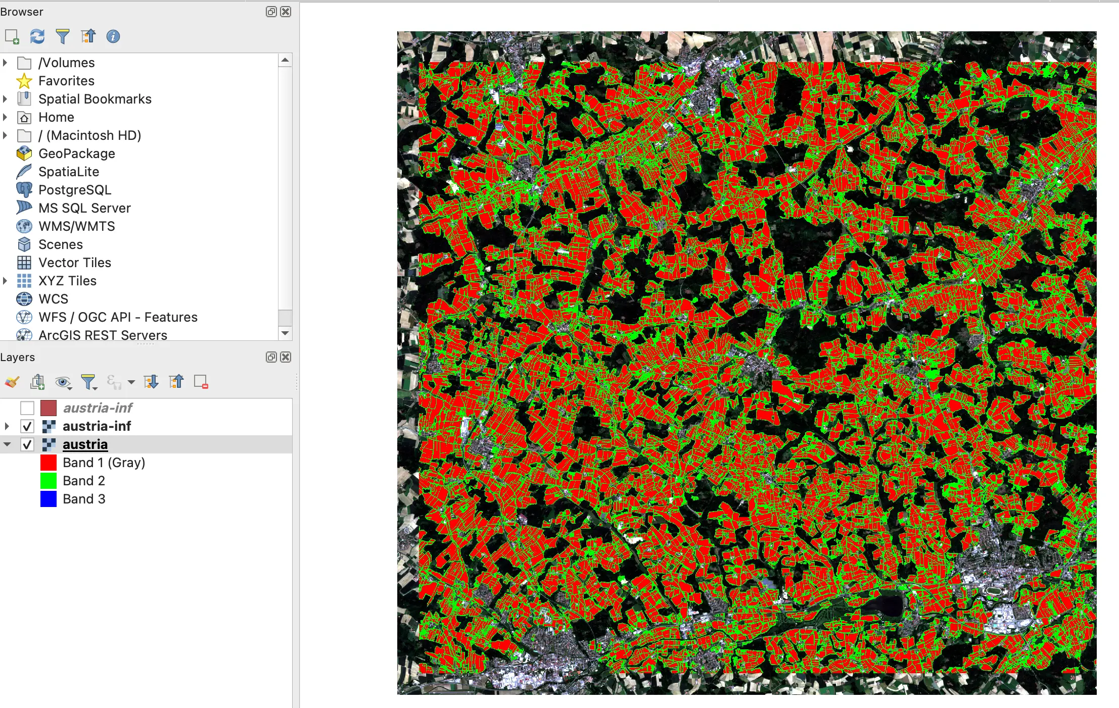
-f -o austria-inf.tif --gpu 0

The output is a GeoTIFF of predicted classes. Use --gpu -1 for CPU (much slower) or --mps_mode on Apple Silicon. The result should look something like this, overlaid on the original imagery in QGIS:

3. Produce Vector Output

Finally, polygonize the raster into vector field boundaries:

ftw inference polygonize austria-inf.tif --simplify 20

This writes austria-inf.parquet, a GeoParquet file following the fiboa specification and including per-parcel area. The simplification factor is in CRS units (meters for Sentinel-2 in UTM); 15–20 usually strikes a good balance between geometry fidelity and file size. Additional options like --min_size, --close_interiors, and the morphological --erode_dilate / --dilate_erode filters let you tune the output. To write other formats (GeoJSON, FlatGeobuf, GeoPackage), pass -o with the matching extension.

If you hit a snag, file an issue describing where things went wrong and we'll help you work through it.

Summary

That's it — field boundaries from satellite imagery, end to end. From here, try the other PRUE variants (FTW_PRUE_EFNET_B3 for speed, FTW_PRUE_EFNET_B7 for accuracy), the Delineate Anything instance-segmentation model, or train your own variant on a custom dataset subset. Results won't be perfect everywhere; improving coverage depends on feedback and contributions from a global community of users. If you've made it this far, we'd love to hear from you — start a discussion with your use case, results, or questions.